
Run enough configurations against the same history and the top row will eventually look exceptional, even if no durable edge exists. That is the central problem of overfitting in trading strategies: confusing the winner of a search with a discovery.
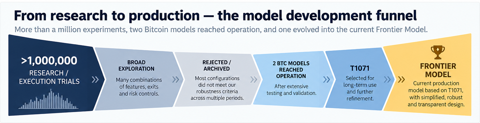
BitcoinAI.Pro has now run more than 1,000,000 machine-learning, execution and robustness trials. Only two Bitcoin generations have crossed from research into operation: the legacy T1071 and the current Frontier Model. The rejection rate is more informative than the prettiest backtest.
The model that learned the sample instead of the market
One of the most useful failures in the research programme was a model whose importance profile exposed a calendar-derived input dominating the decision process. The model had learned when profitable observations occurred in that historical sample rather than a robust market state. It looked good until chronology forced the issue.
The lesson is general: features that let a model index the sample can create convincing backtests without creating durable information. Calendar encodings and other time identifiers therefore receive special scrutiny or are excluded from production tree models.
Why the top row is not a production model
With thousands of trials, a ranking contains both signal and selection luck. The more variants you search, the less meaningful the single best score becomes without independent confirmation.
Our process therefore does not promote a candidate simply because it ranks first. We look for stability across nearby configurations, reproducibility, chronological evidence, repeated-seed robustness where relevant, and behaviour under realistic execution assumptions.
The exact neighbourhood widths, model thresholds and optimisation ranges are not published. They are part of the internal research recipe rather than the methodological lesson.
The current Frontier is not the old eight-input candidate
An earlier version of this article still described the former Frontier branch: eight inputs, a 17,999-trial selection campaign and V83/V84 confirmation statistics. Those are no longer the current production model and should not be presented as such.
The current Frontier is the frozen seven-input BTCUSD D1 XGBoost signal model from the T1071 lineage, with a separately audited execution layer and no automatic production retraining.
Published production inputs
dist_swing_high_12dist_swing_high_24dist_swing_low_12rs_plusrsi_norm_10rv_ratiotsmom_norm
Current evidence, not the retired headline
| Metric | In-sample | Strict model-weight OOS |
|---|---|---|
| Period | Jan 2018 – Jul 2022 | 30 Jul 2022 – Aug 2026 |
| Trades | 151 | 210 |
| SQN | 5.348 | 2.129 |
| Simple return | +733.7 pt | +253.9 pt |
| Win rate | 63.6% | 50.5% |
| Maximum drawdown | -31.04 pt | -25.34 pt |
| Profit / drawdown | 23.63 | 10.02 |
| Research leverage | 1:1 equivalent | 1:1 equivalent |
The uninterrupted V111 full-history replay contains 361 exact trades and ends at +992.65 simple percentage points. The strict model-weight OOS block contains 210 trades, SQN 2.129, +253.9 points, a 50.5% win rate and a maximum drawdown of -25.34 points.
These figures are research statistics at 1:1 notional-equivalent exposure. They are not a compounded live account return and they do not guarantee future results.
Five defences against backtest overfitting
1. Prefer stable regions to isolated peaks
A candidate that works only at one narrow setting is weaker evidence than a broad region with similar behaviour. The principle is public; the exact parameter neighbourhood used internally is not.
2. Reproduce the exact artefact
Before changing a model, reproduce the exact trained binary, input stream and trade sequence. This project only recovered the true T1071 behaviour after treating historical execution semantics as part of the model contract.
3. Keep selection and later evidence separate
A later block stops being independent once it has been inspected repeatedly and used to make decisions. We therefore distinguish historical research OOS from genuinely new forward evidence.
Selection bias is not the only way a backtest can become misleading. Information from future observations can also enter the research process through labels, features or incorrect validation splits. Our guide to data leakage in trading models examines these problems separately from overfitting.
4. Treat retraining as a source of model risk
Repeated refits can sound more adaptive while actually adding variance. In the current Frontier lineage, rolling refits did not justify replacing the exact frozen signal model.
5. Audit execution independently
Signal quality and execution geometry are separate questions. Changing both together makes it impossible to know what produced the apparent improvement. The current Frontier keeps the signal binary frozen while execution research is tested as a separate layer.
What the million-trial number does — and does not — mean
More than one million trials does not make the surviving model true. It means the project has accumulated a very large rejection archive across model, feature, timeframe, execution and robustness experiments.
The important fact is that almost everything was rejected. The two operational BTCUSD generations — T1071 and Frontier Model — are notable because they survived different stages of that process, not because the search count itself proves an edge.
FAQ
What is the difference between overfitting and curve fitting?
Curve fitting describes the behaviour — tuning until history looks good. Overfitting is the statistical consequence: the fitted system has learned the sample more than the underlying process.
How many backtests are too many?
There is no fixed safe number. The larger the search, the more aggressively the selection process must defend against ranking luck and repeated reuse of the same data.
Does walk-forward analysis solve overfitting by itself?
No. Walk-forward is powerful, but it can also be contaminated by repeated tuning, weak sample sizes or a retraining process that is itself unstable.
What details are intentionally withheld?
The public articles disclose the seven input names and aggregate research results. They do not disclose the prediction horizon, target/barrier calibration, decision threshold, exact XGBoost hyperparameters, trained model or complete execution recipe.
Publication boundary. We publish aggregate research results, chronology, validation methodology and the names of the production inputs. We do not publish the target/prediction horizon, label/barrier calibration, decision threshold, exact XGBoost hyperparameters, trained model weights, or the full production execution recipe. Those details are deliberately withheld because they would make the production model substantially easier to reproduce.
See the current AI trading models methodology, the walk-forward worked example, and the public record on BitcoinAI.Pro.
Risk notice. Historical and simulated results are not guarantees of future performance. This article is research, not investment advice.