
Our companion article explains [why the LSTM lost](/lstm-bitcoin-trading-failed/). This one explains why the winner won — because “deep learning didn’t work” is only half a finding. The other half is that a gradient-boosted tree on a small, carefully chosen feature set beat it under identical conditions, and kept beating it after every reasonable attempt to help the network.
**XGBoost for trading** is not a fashionable answer. It is the answer that survives measurement, and there are four structural reasons for that.
## Reason 1: price data is tabular, not sequential
The instinct that price is a sequence and therefore demands a sequence model is intuitive and mostly wrong in practice. Almost everything a recurrent layer can extract from a window of candles — momentum over several horizons, volatility regime, realised-volatility ratios, distance to recent structure, range compression, position within the session — can be computed directly as a feature. Exactly, cheaply, and auditably.
Once those features exist, the model’s job is a tabular classification problem, and gradient-boosted trees are the strongest general-purpose method for tabular problems by a wide margin. You are not throwing away temporal information; you are handing it over pre-digested, so that the model spends its capacity on the decision boundary instead of on rediscovering what a moving average is from a few thousand rows.
## Reason 2: determinism, which is worth more than ceiling
This is the reason that decided our project, and it is almost never mentioned in tutorials.
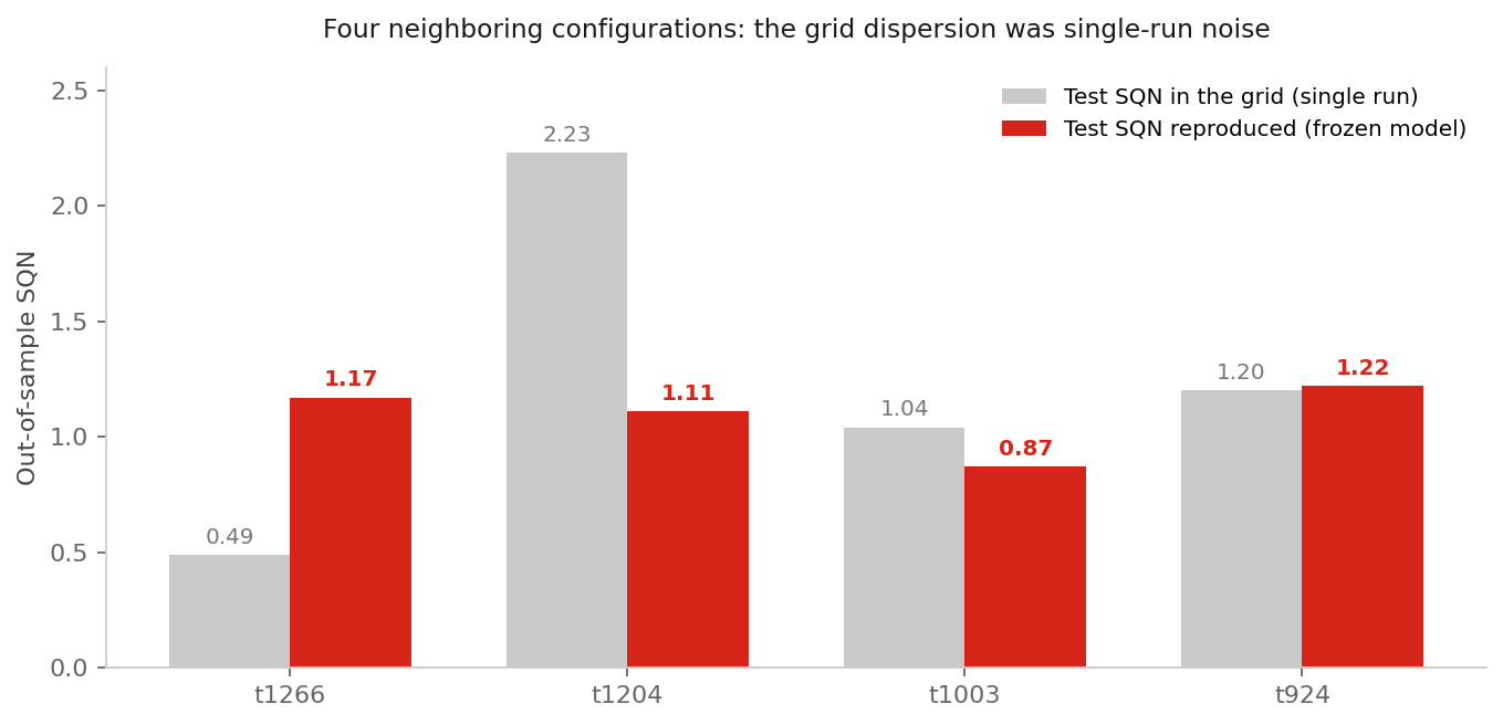
A gradient-boosted tree on fixed features is **reproducible**: same inputs, same model, same score, to the third decimal, twelve rebuilds in a row. The neural alternative was not — identical configurations retrained produced objectives ranging from **0.86 to 4.11**.
Why that matters more than the raw ceiling: research is a comparison process. You run thousands of variants, rank them and promote survivors. If a configuration’s score is itself a random variable with a five-fold spread, the ranking is a ranking of luck, every “improvement” is unmeasured, and a champion is a coincidence with a name. Determinism is what makes the entire validation pipeline — plateau tests, cost stress, reproducibility rebuilds — mean anything at all.
After ensemble averaging stabilised the neural branch enough for a fair comparison, the numbers were **1.79 for the best hybrid against 3.30 for gradient boosting alone**. The tree model won on the metric as well as on the process.
## Reason 3: sample efficiency
Eight years of daily candles is a few thousand rows. Eight years of hourly candles is a few tens of thousands, with a signal-to-noise ratio close to the floor. These are small-data problems by modern standards, and regularised tree ensembles are well behaved on small data in a way that high-capacity sequence models are not.
## Reason 4: interpretability that catches your own mistakes
Split importance is not a truth serum, but it is a smoke alarm. The most valuable diagnostic in our entire project came from an importance chart: a single calendar-derived input absorbing roughly two thirds of a model’s importance. It was not predicting the market — it was memorising *when* profitable trades had occurred in that sample. Removing it lifted validation SQN from 0.88 to 1.66 in one change.
You can build that diagnostic for a neural network too, with more work and less clarity. With a tree model it is one line of code and it fires early.
## The feature set: the eight inputs, named
We publish the composition of the surviving feature set. We do not publish the exact windows, normalisations, thresholds or hyperparameters — those are the part that is expensive to find and cheap to copy. The names are the part that carries the lesson.
The validated index model runs on eight inputs, drawn from four families:
**Volatility regime (2)**
– `atr_ratio` — short-horizon average true range against a longer baseline. Present in the large majority of top-ranked trials across every campaign we have run.
– `rv_ratio` — short-window realised volatility against a long-window baseline. The strongest single feature addition in the history of the project, measured across multiple model versions.
**Realised-volatility decomposition (2)**
– `rs_plus` — upside realised semivariance, the share of realised variance contributed by positive returns.
– `rsj` — relative signed jump variation, the asymmetry between upside and downside realised semivariance. These two are the only inputs in the set that separate *how* volatility was produced from *how much* of it there was.
**Distance to structure (3)**
– `dist_swing_high_12` and `dist_swing_high_24` — normalised distance from price to the recent swing high at two different lookbacks. Two horizons of the same measure survived together, which is itself informative: the model is using the disagreement between them.
– `dist_session_open` — normalised distance from the session open. Together with the swing distances, the most consistently robust input across campaigns on session-based instruments — and, revealingly, close to worthless on 24/7 crypto, which has no session to anchor to. See [Bitcoin vs S&P 500](/bitcoin-vs-sp500-ml-model/).
**Candle geometry (1)**
– `upper_wick_norm` — upper wick normalised by candle range, a rejection measure.
Note what is *not* in there: no oscillator, no moving-average crossover, no trend-strength index, no volume-derived input, and above all no calendar encoding. Eight features, all describing volatility state and position relative to structure.
Three principles govern the set:
**Fewer features, chosen slowly.** Eight inputs, each admitted one at a time against a frozen baseline, is a stronger configuration than thirty added together. Combinatorial feature search over a large pool mostly measures your search budget.
**Importance percentages do not predict what is safe to remove.** Only validation behaviour does. We have removed features carrying 15% of importance with no effect, and removed apparently negligible ones — a volatility z-score with almost no split importance — and watched the model degrade. Ablate; do not infer.
**Anything that lets the model index the sample is banned.** Calendar encodings are the archetype and are permanently excluded from our tree models.
## The cemetery
Just as informative as the surviving set is the list of what was measured and rejected: oscillator histograms, fractal exponents, band-position measures, wick asymmetry, several return z-scores across multiple windows, adaptive trend-strength indices, range-spread measures, a rolling cross-asset correlation, spread estimators derived from high-low ranges, and a variance-risk-premium construction used standalone.
Every one of them was tested one at a time against a frozen baseline, and every one is documented with the reason it lost. That cemetery is why the surviving seven mean something.
Practical notes for building it
- Label with a triple barrier, not with next-bar returns. Take-profit, stop-loss and a time limit, so the label answers the question you actually trade.
- Purge your splits. With overlapping labels, a trade opened near a block boundary resolves across it. See purged cross-validation and data leakage.
- Search with an efficient sampler, decide with a rule. We use Bayesian search over the parameter space, but the promotion criterion is the hidden-block score, never the search objective.
- Never promote the top row. The best trial by validation in one 5,880-trial campaign scored 4.89 in validation and 0.58 on the hidden block. Look for plateaus, not peaks.
- Model costs at the venue’s real commissions, then stress them ×3.
FAQ
Is XGBoost better than LightGBM or CatBoost for trading?
The differences between modern boosting libraries are small compared with the differences made by labelling, splitting and cost modelling. Pick one, and spend the saved effort on validation.
Can XGBoost predict price direction?
It can produce a conditional probability of a barrier being hit first, which is a different and much more tractable question than predicting price. Framing matters more than the algorithm.
How many features should a trading model use?
Fewer than you expect. Our validated index model runs eight — atr_ratio, dist_session_open, dist_swing_high_12, dist_swing_high_24, rs_plus, rsj, rv_ratio, upper_wick_norm — each admitted one at a time against a frozen baseline. Large feature pools mostly enlarge the search space in which overfitting hides.
This article describes methodology and aggregate results. Exact feature definitions, hyperparameters and trained models are not published. Nothing here is investment advice; simulated results are not a guarantee of future performance.